Solving the heat equation in one dimension

This tutorial demonstrates how to numerically solve an equation of the form $$ \frac{\partial y}{\partial t} = f(t, y) $$ using the jax_fno.integrate module. This example demonstrates a typical workflow which goes as follows:

1. Define the (discretised) right-hand-side \(f(t, y)\) of the ODE
2. Set the initial condition \(y_0\)
3. Choose a time-stepping method and integrate

Problem statement

The 1D heat equation is $$ \frac{\partial y}{\partial t} = D \frac{\partial^2 y}{\partial x^2}, $$ where \(D\) is the diffusivity, \(y\) is the temperature at the position \(x\) and time \(t\).

We will solve this with Dirichlet boundary conditions $$ y(t, x=0) = y(t, x=L) = 0, $$ where \(x=0\) and \(x=L\) are the boundaries of the domain.

Starting from a Gaussian initial condition $$ u(t=t_0, x) = \frac{1}{\sqrt{4 \pi D t_0}} \exp^{-x^2 / 4 D t_0}, $$ at time \(t_0\), the diffusion equation has an analytical solution $$ u(t=T, x) = \frac{1}{\sqrt{4 \pi D t}} \exp^{-x^2 / 4 D t} $$ at a later time \(T \geq t_0\).

Spatial discretisation

A uniform finite difference discretisation of the domain leads to interior grid points $$ x_i = i h, \quad i = 1, \ldots, n $$ where the grid spacing \(h = L / (n + 1)\) and \(n\) is the number of interior grid points. We will enforce the boundary conditions by using ghost points at the boundaries.

Implementation

Define the spatial discretisation:

import jax
import jax.numpy as jnp

def laplacian_dirichlet_1d(
    u: jax.Array, 
    bc_left: float, 
    bc_right: float, 
    dx: float
) -> jax.Array:
    """
    Compute the Laplacian (second derivative) using finite differences.
    Assumes ghost points at the boundaries with Dirichlet conditions.
    """
    dudx = jnp.diff(u, prepend=bc_left, append=bc_right)
    return jnp.diff(dudx) / dx**2

def heat_rhs_dirichlet(
    t: float,
    u: jax.Array,
    diffusivity: float,
    bc_left: float,
    bc_right: float,
    dx: float,
) -> jax.Array:
    """Right-hand side of heat equation: du/dt = D d²u/dx²"""
    d2udx2 = laplacian_dirichlet_1d(u, bc_left, bc_right, dx)
    return diffusivity * d2udx2

Set the problem parameters:

# Physical parameters
D = 2.0  # diffusivity
L = 100.0  # domain length
n = 128  # number of grid points
h = L / (n + 1)  # grid spacing
bc_values = (0.0, 0.0)  # Dirichlet boundary condition values

# Time span
t_span = (1.0, 10.0)  # (start_time, end_time)

# Spatial grid (interior points only)
x = jnp.linspace(h, L - h, n, endpoint=True)

Define the initial condition:

def gaussian_ic(x, t, D, L):
    k = 1 / jnp.sqrt(4 * jnp.pi * D * t)
    return k * jnp.exp(-((x - L/2)**2) / (4 * D * t))

y0 = gaussian_ic(x, t_span[0], D, L)

Choose an integration scheme:

from jax_fno.integrate import BackwardEuler, NewtonRaphson, GMRES

linsolver = GMRES(maxiter=50, tol=1e-6)
root_finder = NewtonRaphson(tol=1e-6, maxiter=20, linsolver=linsolver)
method = BackwardEuler(root_finder=root_finder)

Solve:

from jax_fno.integrate import solve_ivp

t_final, y_final = solve_ivp(
    heat_rhs_dirichlet,
    t_span,
    y0,
    method,
    step_size=1e-1,
    args=(D, bc_values[0], bc_values[1], h)
)

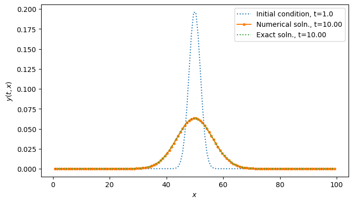
Visualise the results:

import matplotlib.pyplot as plt

yT_exact = gaussian_ic(x, t_span[1], D, L)

fig, ax = plt.subplots(figsize=(8, 4.5))
ax.plot(x, y0, ':', label=f"Initial condition, t={t_span[0]}")
ax.plot(x, y_final, '-', marker='.', label=f"Numerical soln., t={t_final:.2f}")
ax.plot(x, yT_exact, ':', label=f"Exact soln., t={t_span[1]:.2f}")
ax.legend()
ax.set_xlabel('$x$')
ax.set_ylabel('$y(t, x)$')
plt.show()