Implicit solver for the heat equation

This tutorial demonstrates how to numerically solve an equation of the form \(\partial u / \partial t = f(t, u)\) using pardax. It covers spatial discretisation, the solver pipeline, and implicit time stepping.

Problem statement

The 1D heat equation is

\[ \frac{\partial u}{\partial t} = D \frac{\partial^2 u}{\partial x^2}, \]

where \(D\) is the diffusivity and \(u(t, x)\) is the temperature at position \(x\) and time \(t\).

We solve on \(x \in [0, L]\) with homogeneous Dirichlet boundary conditions

\[ u(t, 0) = u(t, L) = 0. \]

Starting from a Gaussian centred at \(x = L/2\),

\[ u(t_0, x) = \frac{1}{\sqrt{4 \pi D t_0}} \exp\!\left(-\frac{(x - L/2)^2}{4 D t_0}\right), \]

the heat equation has the analytical solution

\[ u(t, x) = \frac{1}{\sqrt{4 \pi D t}} \exp\!\left(-\frac{(x - L/2)^2}{4 D t}\right) \]

for \(t \geq t_0\), which we will use to verify the numerical result.

1. Spatial discretisation

We use a uniform finite difference grid with \(n\) interior points

\[ x_i = i \, \Delta x, \quad i = 1, \ldots, n, \]

where \(\Delta x = L / (n + 1)\). The boundary values \(u = 0\) at \(x = 0\) and \(x = L\) are enforced through ghost points in the Laplacian stencil.

import jax
import jax.numpy as jnp

def laplacian_dirichlet_1d(u, bc_left, bc_right, dx):
    """Second-order central difference Laplacian with Dirichlet BCs."""
    dudx = jnp.diff(u, prepend=bc_left, append=bc_right)
    return jnp.diff(dudx) / dx**2

def heat_rhs(t, u, params):
    """Right-hand side: du/dt = D * d²u/dx²."""
    return params["D"] * laplacian_dirichlet_1d(
        u, params["bc_left"], params["bc_right"], params["dx"]
    )

The right-hand side function must have the signature fun(t, y, params) -> dy/dt. Any additional parameters (D, bc_left, etc.) are passed as a single params pytree when calling solve_ivp.

2. Parameters and initial condition

# Physical parameters
D = 2.0       # diffusivity
L = 50.0     # domain length
n = 128       # number of interior grid points
dx = L / (n + 1)

# Boundary conditions
bc_left, bc_right = 0.0, 0.0

# Spatial grid (interior points only)
x = jnp.linspace(dx, L - dx, n, endpoint=True)

def gaussian(x, t, D, L):
    return jnp.exp(-((x - L/2)**2) / (4*D*t)) / jnp.sqrt(4*jnp.pi*D*t)

t_span = (1.0, 10.0)

y0 = gaussian(x, t_span[0], D, L)

3. Build the solver and integrate

In pardax, implicit time stepping is assembled from composable components:

1. A linear solver (AbstractLinearSolver) solves the linear system that arises at each Newton iteration.
2. A lineariser (AbstractLineariser) constructs a linear system from the nonlinear residual, using automatic differentiation or a user-supplied Jacobian.
3. A root finder (AbstractRootFinder) drives the outer Newton iteration to convergence.
4. A time stepper (AbstractStepper) defines the implicit residual and delegates to the root finder.

import pardax as pdx

linsolver = pdx.GMRES(tol=1e-6, maxiter=50)

root_finder = pdx.NewtonRaphson(
    lineariser=pdx.AutoJVP(linsolver=linsolver),
    tol=1e-6,
    maxiter=20,
)

method = pdx.BackwardEuler(root_finder=root_finder)

Because backward Euler is unconditionally stable for the heat equation, we can use a time step much larger than the explicit diffusive CFL limit \(\Delta t \lesssim \Delta x^2 / (2D)\):

t, y = pdx.solve_ivp(
    heat_rhs,
    t_span=t_span,
    y0=y0,
    stepper=method,
    step_size=1e-1,
    params={"D": D, "bc_left": bc_left, "bc_right": bc_right, "dx": dx},
    num_checkpoints=2,
)

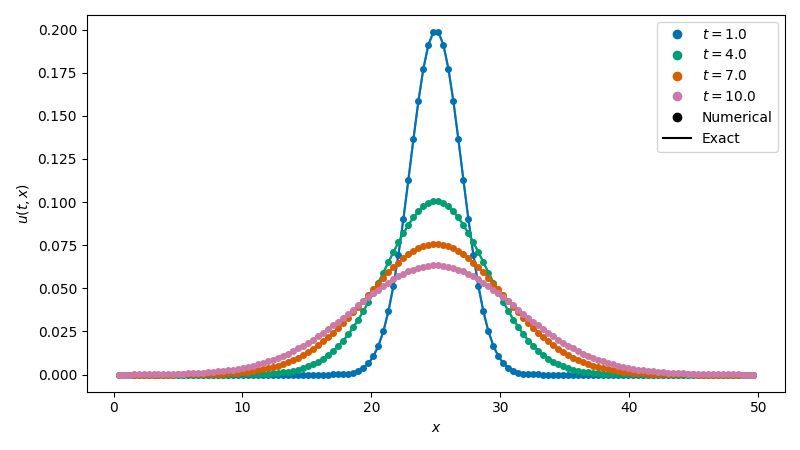
4. Visualise the results

import matplotlib.pyplot as plt
import matplotlib.cm as cm

fig, ax = plt.subplots(figsize=(8, 4.5), layout='tight')

norm = plt.Normalize(vmin=t.min(), vmax=t.max())  # type: ignore
cmap = cm.viridis  # type: ignore

for i in range(len(t)):
    c = cmap(norm(t[i]))
    ax.plot(x, y[i], marker='o', color=c, markersize=4, ls='none')
    ax.plot(x, gaussian(x, t[i], D, L), ls='-', color=c, alpha=0.7)

# Style-only legend entries in neutral grey
grey = '0.3'
ax.plot([], [], marker='o', ls='none', color=grey, label='Numerical')
ax.plot([], [], ls='-', color=grey, alpha=0.7, label='Exact')
ax.legend(fontsize=11)

sm = cm.ScalarMappable(cmap=cmap, norm=norm)
cbar = fig.colorbar(sm, ax=ax)
cbar.set_label("$t$", fontsize=11)

ax.set_xlabel("$x$", fontsize=11)
ax.set_ylabel("$u(t, x)$", fontsize=11)

plt.show()