Generating training data on Burgers' equation in 1D

This tutorial demonstrates how a training dataset for Burgers' equation in 1D is generated. Users that just want to run a generation script without reading this tutorial can look at examples/burgers1d/generate.py on GitHub.

Note: This tutorial requires users to have h5py and pardax installed.

Problem statement

The 1D viscous Burgers' equation on a periodic domain \(x \in [0, 1)\) reads

\[ \frac{\partial u}{\partial t} = -u\frac{\partial u}{\partial x} + \nu\frac{\partial^2 u}{\partial x^2}, \]

where \(\nu > 0\) is the kinematic viscosity. The task is to generate input-output pairs \(u_0(x) = u(x, t=0)\) and \(u(x, t=1)\), where the initial conditions are drawn from a Gaussian random field:

\[ u_0 \sim \mathcal{N}\!\left(0,\; 625(-\Delta + 25I)^{-2}\right), \]

where \(\Delta\) is the Laplacian.

Setup

import h5py
import jax
import jax.numpy as jnp
import numpy as np
import equinox as eqx
import pardax as pdx

nu = 0.02  # Kinematic viscosity
L = 1.0  # Domain length
resolution = 256  # Number of grid points
dx = L / resolution  # Grid spacing
x = np.linspace(0, L, num=resolution, endpoint=False)  # Grid points

Initial conditions

Initial conditions are sampled from a Gaussian random field. In Fourier space, the Laplacian is diagonal with eigenvalues \(-k^2\), where \(k\) is the wavevector.

class GaussianField1D(eqx.Module):
    """Sample 1D fields from N(0, 625(-Δ + 25I)^{-2}) on a periodic grid."""

    coef: jax.Array
    k: jax.Array
    n: int
    L: float

    def __init__(self, n: int, L: float) -> None:
        self.n = n
        self.L = L
        k = 2 * jnp.pi * jnp.fft.fftfreq(n, d=L / n)
        self.k = k
        self.coef = jnp.sqrt(625 * (k**2 + 25) ** (-2))

    def sample(self, key: jax.Array) -> jax.Array:
        n = self.n
        coef = self.coef

        key_dc, key_re, key_im, key_nyq = jax.random.split(key, 4)
        dc = jax.random.normal(key_dc, (1,))

        m = (n - 1) // 2
        re_int = jax.random.normal(key_re, (m,))
        im_int = jax.random.normal(key_im, (m,))
        interior_modes = (re_int + 1j * im_int) / jnp.sqrt(2.0)

        if n % 2 == 0:
            nyquist = jax.random.normal(key_nyq, (1,))
            pos = jnp.concatenate([dc, interior_modes, nyquist])
        else:
            pos = jnp.concatenate([dc, interior_modes])

        neg = jnp.conj(jnp.flip(pos[1 : m + 1]))
        noise = jnp.concatenate([pos, neg])

        f_k = coef * noise
        f_x = jnp.fft.ifft(f_k) * n
        return jnp.real(f_x)

Set up the random field sampler and a batched sampling function:

num_samples = 1280
batch_size = 64
key = jax.random.key(0)
grf = GaussianField1D(resolution, L)

sample_batch = jax.vmap(jax.jit(lambda key_: grf.sample(key_)))

Numerical solver

The spatial derivatives are discretised using second-order accurate central differences.

The advection and diffusion right-hand sides are defined as:

def advection(t: float, u: jax.Array, nu: float, dx: float) -> jax.Array:
    """-u * du/dx (periodic, central differences)."""
    dudx = (jnp.roll(u, -1) - jnp.roll(u, 1)) / (2 * dx)
    return -u * dudx


def diffusion(t: float, u: jax.Array, nu: float, dx: float) -> jax.Array:
    """nu * d²u/dx² (periodic, central differences)."""
    return nu * (jnp.roll(u, -1) - 2 * u + jnp.roll(u, 1)) / dx**2

The solution is advanced through time with an implicit-explicit (IMEX) scheme. The advective term is advanced with a forward Euler method and the diffusive term is advanced with a backward Euler method.

The linear system resulting from the discretisation of the diffusive term is diagonalised in Fourier space using the eigenvalues \(\sigma_k\) of the second-order central difference stencil on a periodic grid, where

\[ \sigma_k = \frac{-4\sin^2(k\Delta x/2)}{\Delta x^2}. \]

The implicit system at each time step reduces to a pointwise division in frequency space rather than a full linear solve.

k = 2 * jnp.pi * jnp.fft.rfftfreq(resolution, d=dx)
sigma = -4 * nu * jnp.sin(k * dx / 2) ** 2 / dx**2

operator = pdx.SpectralOperator(eigvals=sigma)

spectral_solver = pdx.SpectralSolver(
    forward=jnp.fft.rfft,
    backward=lambda x: jnp.fft.irfft(x, n=resolution),
)

root_finder = pdx.LinearRootFinder(
    linsolver=spectral_solver,
    operator=operator
)

stepper = pdx.IMEX(
    explicit=pdx.ForwardEuler(),
    implicit=pdx.BackwardEuler(root_finder=root_finder),
)

For further details on numerical time integration in JAX, check out pardax or diffrax.

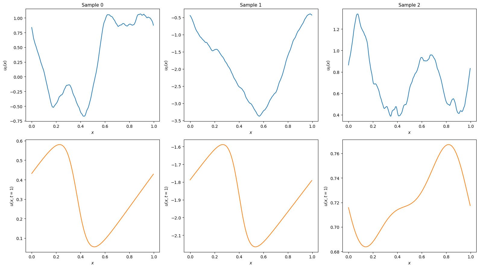
Solving the PDE

Define the RHS dictionary and a batched solver:

rhs = {"explicit": advection, "implicit": diffusion}

dt = 1e-4  # time step size
t_end = 1.0

solve_batch = jax.vmap(
    jax.jit(
        lambda y0: pdx.solve_ivp(
            rhs,
            (0.0, t_end),
            y0,
            stepper,
            dt,
            args=(nu, dx),
        )
    )
)

Visualise a few samples to confirm the setup looks right:

import matplotlib.pyplot as plt

num_examples = 3
key, subkey = jax.random.split(key)
preview_keys = jax.random.split(subkey, num_examples)
y0_preview = sample_batch(preview_keys) # (num_examples, resolution)

_, y_preview = solve_batch(y0_preview)  # (num_examples, T+1, resolution)
y_end_preview = y_preview[:, -1, :]  # (num_examples, resolution)

fig, axes = plt.subplots(2, num_examples, figsize=(16, 9), layout="tight")

for i in range(num_examples):
    axes[0, i].plot(x, y0_preview[i], color='C0')
    axes[0, i].set_xlabel("$x$", fontsize=10)
    axes[0, i].set_ylabel("$u_0(x)$", fontsize=10)
    axes[0, i].set_title(f"Sample {i}", fontsize=11)

    axes[1, i].plot(x, y_end_preview[i], color='C1')
    axes[1, i].set_xlabel("$x$", fontsize=10)
    axes[1, i].set_ylabel("$u(x, t=1)$", fontsize=10)

plt.show()

Generating and saving the dataset

Rather than solving for all samples at once, we generate and write in batches to keep peak memory usage bounded. The HDF5 datasets are pre-allocated with the full shape and filled slice-by-slice.

First, infer the dtype from a single probe sample:

key, subkey = jax.random.split(key)
_y0_probe = grf.sample(subkey)
dtype = np.asarray(_y0_probe).dtype

Then create the HDF5 file and fill it batch by batch:

output_path = "myburgersdataset.h5"

with h5py.File(output_path, "w") as f:
    ds_in = f.create_dataset(
        "inputs",
        shape=(num_samples, resolution, 2),
        dtype=dtype,
        chunks=(min(batch_size, num_samples), resolution, 2),
    )
    ds_out = f.create_dataset(
        "outputs",
        shape=(num_samples, resolution, 1),
        dtype=dtype,
        chunks=(min(batch_size, num_samples), resolution, 1),
    )

    ds_in.attrs["description"] = (
        "[sample, :, 0] = grid points x, "
        "[sample, :, 1] = initial condition u_0(x)"
    )
    ds_out.attrs["description"] = "[sample, :, 0] = solution u(x, t_end)"

    f.attrs.update(
        {
            "nu": nu,
            "dt": dt,
            "t_end": t_end,
            "resolution": resolution,
            "num_samples": num_samples,
            "L": L,
        }
    )

    for start in range(0, num_samples, batch_size):
        end = min(start + batch_size, num_samples)
        batch = end - start

        key, subkey = jax.random.split(key)
        batch_keys = jax.random.split(subkey, batch)
        y0 = sample_batch(batch_keys)  # (batch, resolution)

        _, y = solve_batch(y0)  # (batch, T+1, resolution)
        y_end = y[:, -1, :]  # (batch, resolution)

        inputs_np = np.empty((batch, resolution, 2), dtype=dtype)
        inputs_np[:, :, 0] = x[None, :]
        inputs_np[:, :, 1] = np.asarray(y0)

        ds_in[start:end] = inputs_np
        ds_out[start:end] = np.asarray(y_end)[:, :, None]

        print(f"  {end}/{num_samples} samples written")

print(f"Dataset saved to {output_path}")

  64/1280 samples written
  128/1280 samples written
  192/1280 samples written
  ...
  1216/1280 samples written
  1280/1280 samples written
Dataset saved to myburgersdataset.h5