Training an FNO on Burgers' equation in 1D

This example demonstrates how a Fourier neural operator can be trained to predict solutions of Burgers' equation in 1D.

Users that want to just run a training script without reading this tutorial can look at examples/burgers1d/train.py on GitHub.

Note: This tutorial requires users to have datasets, optax, matplotlib installed.

Problem statement

Burgers' equation in 1D on a periodic domain \(x \in [0, 1)\) reads

\[ \frac{\partial u}{\partial t} = -u\frac{\partial u}{\partial x} + \nu\frac{\partial^2 u}{\partial x^2}, \]

where \(\nu > 0\) is the kinematic viscosity. The first term is a non-linear advective term and the second is a diffusive term.

The learning task is to approximate the solution operator

\[ \mathcal{G}^{\dagger} : u_0 \mapsto u\left(\cdot, t_{\text{end}}\right) \]

mapping an initial condition \(u_0\) to the solution at time \(t_{\text{end}}\).

import math
import json
from functools import partial

import norax as nrx
import datasets
import jax
import jax.numpy as jnp
import numpy as np
import optax
import equinox as eqx

Data loading

Load the data from Hugging Face:

ds = datasets.load_dataset("TortillaChip/burgers1d-periodic", split="train")

To generate the data yourself, see the Generating Training Data example.

Data preprocessing

def preprocess(ds: datasets.Dataset, stride: int = 1):
    """Build ``input`` and ``output`` columns.

    The resulting input column stacks the spatial grid and initial condition
    along the last axis. The resulting output column is reshaped to have a
    size-1 dimension as its last axis. 

    Optionally downsample the spatial grid with stride.
    """

    out_features = datasets.Features(
        {
            "input": datasets.Array2D(shape=(target_res, 2), dtype="float32"),
            "output": datasets.Array2D(shape=(target_res, 1), dtype="float32"),
        }
    )

    def _build(batch):
        x = np.array(batch["x"])[:, ::stride]
        u0 = np.array(batch["u0"])[:, ::stride]
        u_T = np.array(batch["u_end"])[:, ::stride]
        return {"input": np.stack([x, u0], axis=-1), "output": u_T[:, :, None]}

    return ds.map(
        _build,
        batched=True,
        remove_columns=ds.column_names,
        features=out_features,
    ).with_format("jax")

orig_res = 8192  # original resolution
target_res = 256  # target resolution
stride = orig_res // target_res
nu = 0.2  # viscosity
t_end = 1.0  # end time

ds = preprocess(ds, stride)

Split the data into train and test sets:

splits = ds.train_test_split(test_size=0.2, shuffle=False)

train_ds = splits["train"]
test_ds = splits["test"]

Model

key = jax.random.key(0)
key, subkey = jax.random.split(key)

model = nrx.FNO(
    key=subkey,
    channels_in=2,
    channels_out=1,
    n_modes=(16,),
    width=64,
    depth=4,
)

print(model)

nrx.FNO(
  lift=MLP(
    activation=<function gelu>,
    depth=2,
    width=128,
    hidden_layers=(Linear(weight=f32[128,2], bias=f32[128]),),
    output_layer=Linear(weight=f32[64,128], bias=f32[64])
  ),
  project=MLP(
    activation=<function gelu>,
    depth=2,
    width=128,
    hidden_layers=(Linear(weight=f32[128,64], bias=f32[128]),),
    output_layer=Linear(weight=f32[1,128], bias=f32[1])
  ),
  fourier_layers=(
    Fourier(
      spectral=SpectralConv(
        channels_in=64,
        channels_out=64,
        n_modes=(16,),
        n_dims=1,
        weights_re=f32[64,64,16],
        weights_im=f32[64,64,16]
      ),
      linear=Linear(weight=f32[64,64], bias=f32[64]),
      activation=<function gelu>
    ),
    ...
  )
)

Verify that a forward pass works for a couple of samples:

batch = next(iter(train_ds.iter(batch_size=2)))
jax.vmap(model)(batch["input"]).shape

(2, 64, 1)

Evaluation

def relative_l2(prediction: jax.Array, target: jax.Array) -> jax.Array:
    return jnp.linalg.norm(prediction - target) / jnp.linalg.norm(target)


@partial(jax.vmap, in_axes=(None, 0, 0))
def loss_fn(model: nrx.FNO, x: jax.Array, y: jax.Array) -> jax.Array:
    return relative_l2(model(x), y)


@jax.jit
def eval_step(model: nrx.FNO, x: jax.Array, y: jax.Array) -> jax.Array:
    return jnp.sum(loss_fn(model, x, y))


def evaluate(model: nrx.FNO, dataset: datasets.Dataset, batch_size: int) -> float:
    total_loss = jnp.zeros(())
    n_samples = 0
    for batch in dataset.iter(batch_size=batch_size):
        x, y = batch["input"], batch["output"]
        n_samples += x.shape[0]
        total_loss += eval_step(model, x, y)
    return float(total_loss / n_samples)

Training

Create an Adam optimiser with a learning rate that halves every 100 epochs:

learning_rate = 1e-3
batch_size = 32
steps_per_epoch = math.ceil(len(train_ds) / batch_size)

schedule = optax.schedules.exponential_decay(
    learning_rate,
    transition_steps=steps_per_epoch * 100,
    decay_rate=0.5,
    staircase=True,
)

optimiser = optax.adam(schedule)
opt_state = optimiser.init(eqx.filter(model, eqx.is_array))

Define a single training step (batch update):

@eqx.filter_jit
def train_step(
    model: nrx.FNO,
    opt_state: optax.OptState,
    optimiser: optax.GradientTransformation,
    x: jax.Array,
    y: jax.Array,
):
    loss, grads = eqx.filter_value_and_grad(
        lambda m: jnp.mean(loss_fn(m, x, y))
    )(model)
    updates, opt_state = optimiser.update(
        grads, opt_state, eqx.filter(model, eqx.is_array)
    )
    model = eqx.apply_updates(model, updates)
    return model, opt_state, loss * x.shape[0]

Define a training epoch. The dataset is shuffled with a fresh seed each epoch by calling .shuffle() before iterating:

def run_epoch(
    model: nrx.FNO,
    opt_state: optax.OptState,
    optimiser: optax.GradientTransformation,
    ds: datasets.Dataset,
    batch_size: int,
):
    total_loss = jnp.zeros(())
    n_samples = 0
    for batch in ds.iter(batch_size=batch_size):
        x, y = batch["input"], batch["output"]
        n_samples += x.shape[0]
        model, opt_state, batch_loss = train_step(
            model, opt_state, optimiser, x, y
        )
        total_loss += batch_loss
    return model, opt_state, float(total_loss / n_samples)

Run the training loop:

n_epochs = 500

for epoch in range(1, n_epochs + 1):
    shuffled = train_ds.shuffle(seed=epoch)
    model, opt_state, train_loss = run_epoch(
        model, opt_state, optimiser, shuffled, batch_size
    )

    if epoch % 10 == 0 or epoch == n_epochs:
        test_loss = evaluate(model, test_ds, batch_size)
        print(
            f"Epoch {epoch:4d}/{n_epochs}  "
            f"train={train_loss:.4e}  test={test_loss:.4e}"
        )

Epoch   10/500  train=1.0623e-01  test=9.8970e-02
Epoch   20/500  train=6.6438e-02  test=6.6549e-02
Epoch   30/500  train=3.9810e-02  test=3.8570e-02
...

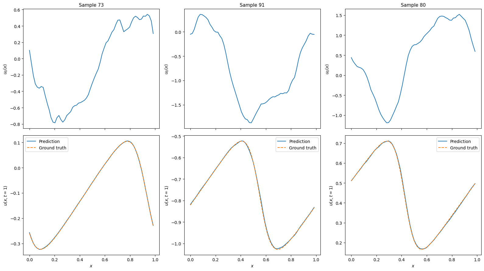
Predictions

import matplotlib.pyplot as plt

num_examples = 3

key = jax.random.key(0)
key, subkey = jax.random.split(key)
random_inds = jax.random.choice(
    subkey, len(test_ds), (num_examples,), replace=False
).tolist()

examples = test_ds.select(random_inds)[:]
example_inputs = examples["input"]
example_outputs = examples["output"]
predictions = jax.vmap(model)(example_inputs)

fig, axes = plt.subplots(
    2, num_examples, figsize=(16, 9), layout="tight", sharex=True
)

for i in range(num_examples):
    x = example_inputs[i, :, 0]
    u0 = example_inputs[i, :, 1]
    v_true = example_outputs[i, ...]
    v_pred = predictions[i, ...]

    axes[0, i].plot(x, u0)
    axes[0, i].set_ylabel("$u_0(x)$", fontsize=10)
    axes[0, i].set_title(f"Sample {random_inds[i]}", fontsize=11)

    axes[1, i].plot(x, v_pred, "-", label="Prediction")
    axes[1, i].plot(x, v_true, "--", label="Ground truth")
    axes[1, i].set_xlabel("$x$", fontsize=10)
    axes[1, i].set_ylabel("$u(x, t=1)$", fontsize=10)
    axes[1, i].legend(fontsize=10)

plt.show()

Saving and loading models

def save_model(path: str, model: nrx.FNO, hyperparams: dict) -> None:
    """Save model weights and hyperparameters to a binary file.

    The file format follows the Equinox recommended pattern:
    a JSON-encoded hyperparameter line followed by the serialised leaves.
    """
    with open(path, "wb") as f:
        f.write((json.dumps(hyperparams) + "\n").encode())
        eqx.tree_serialise_leaves(f, model)


def load_model(path: str):
    """Load a model previously saved with `save_model`."""
    with open(path, "rb") as f:
        hyperparams = json.loads(f.readline().decode())
        hyperparams["n_modes"] = tuple(hyperparams["n_modes"])
        skeleton = nrx.FNO(key=jax.random.key(0), **hyperparams)
        model = eqx.tree_deserialise_leaves(f, skeleton)
    return model, hyperparams

hyperparams = {
    "channels_in": 2,
    "channels_out": 1,
    "n_modes": list((16,)),
    "width": 64,
    "depth": 4,
}

save_model("mymodel.eqx", model, hyperparams)
print("Model saved.")

# Verify that saving and loading works
model_loaded, hyperparams_loaded = load_model("mymodel.eqx")
print("Model loaded. hyperparams:", hyperparams_loaded)

Model saved.
Model loaded. hyperparams: {'channels_in': 2, 'channels_out': 1, 'n_modes': (16,), 'width': 64, 'depth': 4}